2  Operating Models

2.1 OM Conditioning

The 2023 ISC stock assessment of North Pacific swordfish, which was fitted with Stock Synthesis 3 (SS3; Methot and Wetzel (2013)), was used to generate the operating models (OMs).

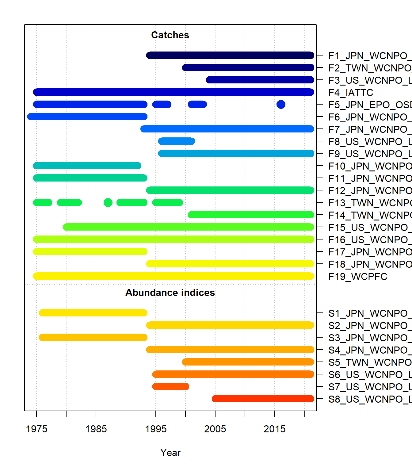
The assessment is a two-sex model with 4 quarterly time steps per year, covering 1975–2021. It includes 19 fishing fleets and 8 CPUE indices (Figure 2.1; Table 2.1). Steepness of the Beverton-Holt stock-recruitment relationship is fixed at 0.9. See the assessment report for further details on the assessment structure and assumptions.

The OMs were constructed by importing the SS3 output of each assessment run, available from the WCNPOSWO-2023 repository, into the North Pacific swordfish MSE framework.

Figure 2.1: Overview of the data used in the 2023 base case stock assessment.

2.1.1 Catch Units

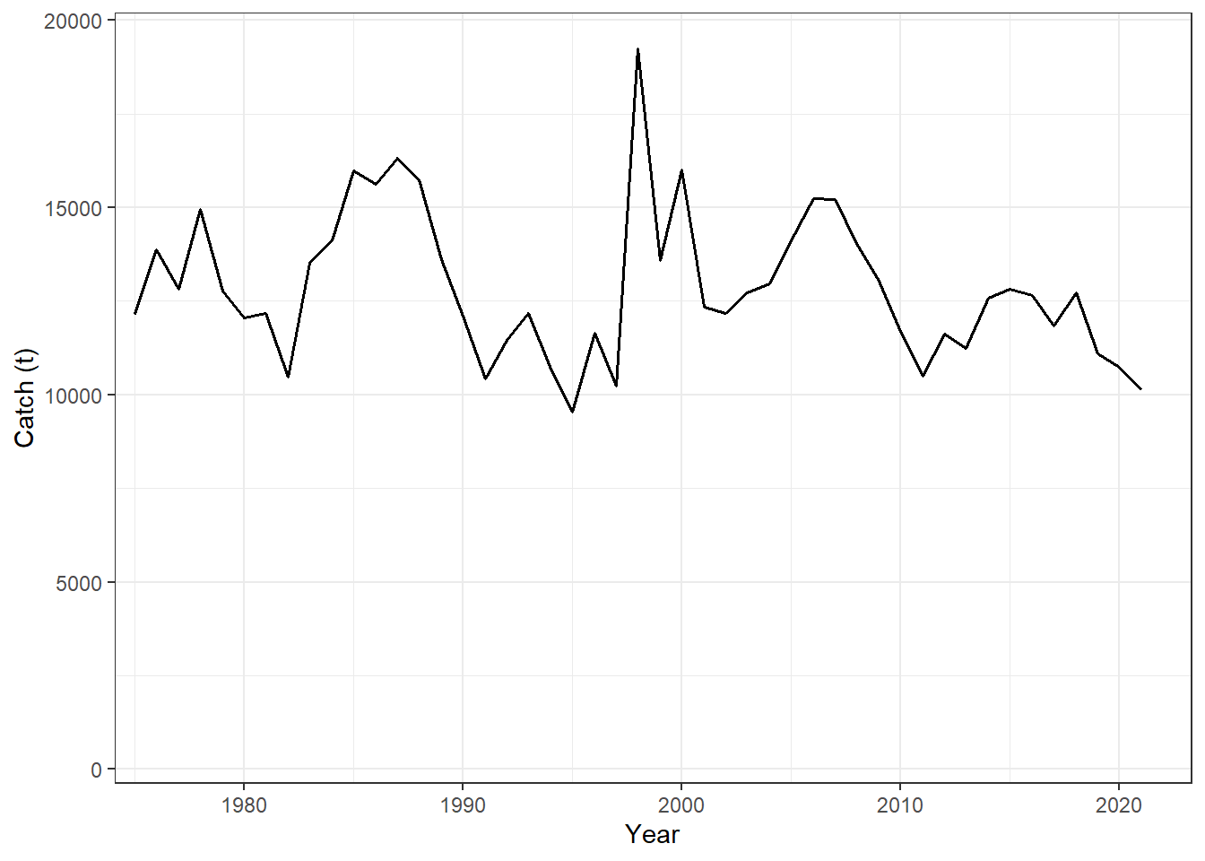
In the assessment, the catch of 8 of the 19 fishing fleets is in numbers of fish (thousands), and the catch of the remaining fleets is in biomass (t). Because the total allowable catch (TAC) management advice produced by the candidate management procedures (CMPs) is in units of biomass (tons), the catch of every fleet was imported in biomass, using the catch biomass predicted by SS3 for the fleets with catch in numbers.

2.1.2 Fleet Structure

To reduce run time, the 19 fishing fleets were combined into a single fleet in the operating models. The combined fleet reproduces the historical fishing mortality-at-age of the individual fleets, with selectivity, retention, and weight-at-age weighted by the fishing mortality of each fleet. This results in exactly the same fishery and population dynamics as an operating model that includes the 19 fleet structure. In the projection period, the relative contribution of each fleet (i.e., TAC allocation) is therefore assumed to be fixed at its recent pattern.

Figure 2.2: Total annual catch data in the base case OM.

2.1.3 Indices of Abundance

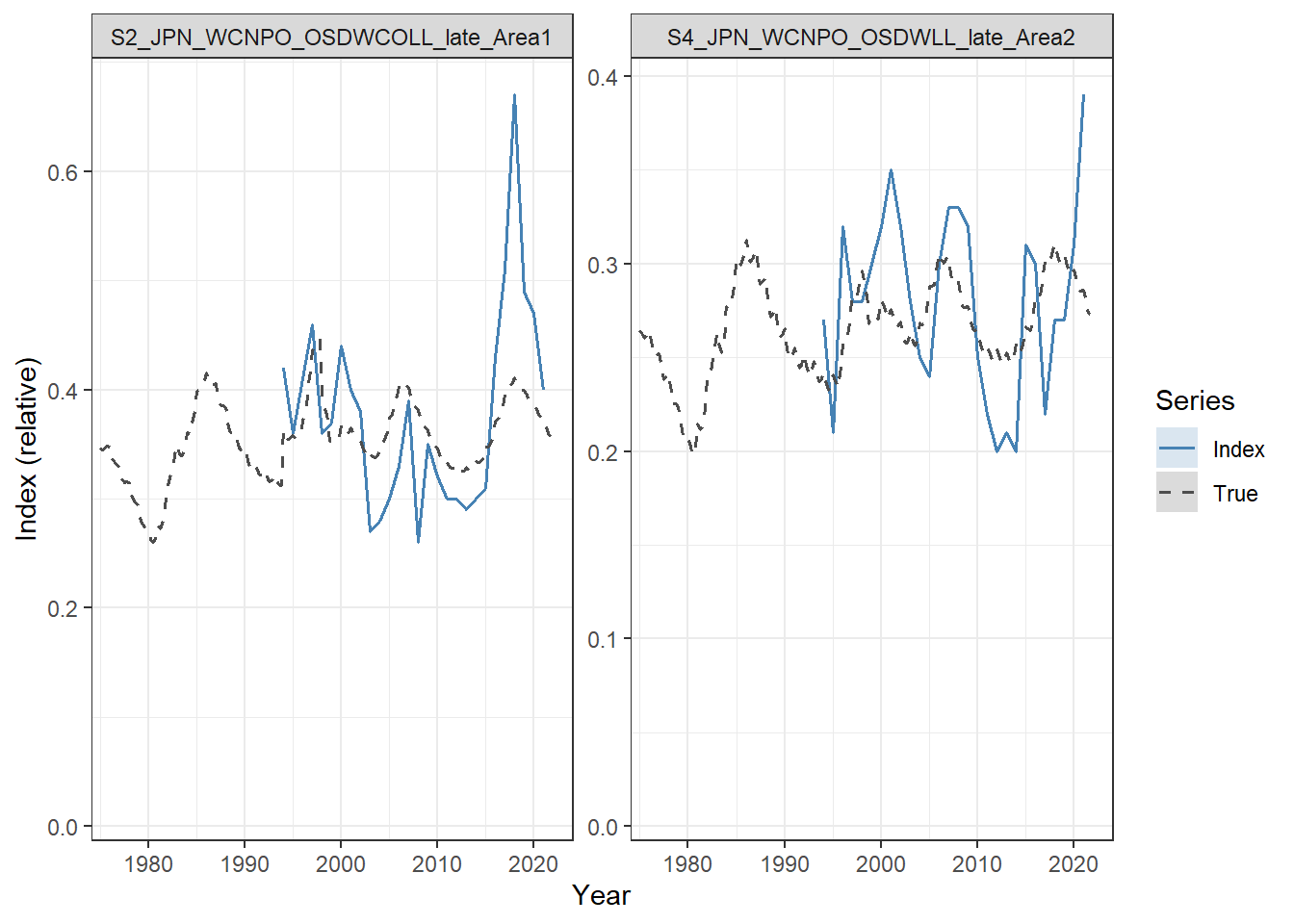
Table 2.1 lists the CPUE indices in the assessment. The Japanese longline indices (Area 1 and Area 2; both split into an Early and Late phase) were selected to be used by the CMPs.

The index-based CMPs use the two that continue to the terminal year (S2 and S4; Figure 2.3). The surplus production CMPs also use the earlier Japanese longline series (S1 and S3; see Chapter 5).

Two of the indices (S5 and S8) were not fitted in the base case assessment (lambda = 0), and therefore were not included in the data passed to the CMPs.

S6, an index of recruitment, was also not used by the CMPs. This index has a higher CV than the Japanese longline indices, and as it does not track the adult population it did not provide any additional information that could improve the performance of the CMPs.

Table 2.1: The CPUE indices in the base case assessment, the years with data, the units, the lambda (weight in the likelihood) in the base case assessment, and the CMPs that use each index.

Index	Years	Units	SS3 lambda	Used by CMPs
S1_JPN_WCNPO_OSDWLL_early_Area1	1976–1993	Number	1	SP
S2_JPN_WCNPO_OSDWCOLL_late_Area1	1994–2021	Number	1	IR, IT, SP
S3_JPN_WCNPO_OSDWLL_early_Area2	1976–1993	Number	1	SP
S4_JPN_WCNPO_OSDWLL_late_Area2	1994–2021	Number	1	IR, IT, SP
S5_TWN_WCNPO_DWLL_late	2000–2021	Number	0
S6_US_WCNPO_LL_deep	1995–2021	Recruitment	1
S7_US_WCNPO_LL_shallow_early	1995–2000	Number	1
S8_US_WCNPO_LL_shallow_late	2005–2021	Number	0

Figure 2.3: The two Japanese longline indices used by the index-based CMPs (S2: Area 1, S4: Area 2) and the corresponding vulnerable abundance in the base case OM. The model-based surplus production CMPs also used the earlier phases of these two indices (S1 and S3).

2.2 Base Case and Sensitivity OMs

2.2.1 OMs Included in the MSE

The 2023 assessment included sensitivity runs with alternative life-history parameters (natural mortality, steepness, growth, and maturity), catch assumptions, model settings, and CPUE indices. OMs were constructed from the base case and the 9 sensitivity runs with alternative life-history parameters (Table 2.2; Table 2.3). The other sensitivity runs are not currently included in the MSE.

Three of these runs are not included in the MSE:

• Run 03 (steepness 0.70): the control file sets steepness to 0.70, but the starter file initialises the parameters from the base case parameter file, where steepness is 0.9. Because steepness is fixed, the fitted model has steepness of 0.9 and the SS3 output is identical to the base case, so the run does not represent the steepness sensitivity.
• Runs 05 (steepness 0.99) and 06 (maximum size 10% larger): the SS3 fits estimate an implausibly large stock, with ln(R0) of 32.37 and 35.06 compared with 6.84 in the base case, and unfished spawning biomass of the order of \(10^{16}\) and \(10^{17}\) t. The stock in these OMs is therefore effectively unfished and unaffected by the catch.

The CMPs are tuned on the base case OM (Section 5.7) and their robustness is evaluated on the 6 included sensitivity OMs.

Table 2.2: The SS3 runs of the 2023 assessment used to construct OMs, and whether each OM is included in the MSE.

OM	Description	Included	Reason for exclusion
00	Base Case	Yes
01	M 10% lower	Yes
02	M 10% higher	Yes
03	Steepness 0.70	No	Output identical to base case
04	Steepness 0.81	Yes
05	Steepness 0.99	No	Implausibly large stock
06	Maximum size 10% larger	No	Implausibly large stock
07	Growth from Sun et al. (2002)	Yes
08	L50 10% higher	Yes
09	L50 10% lower	Yes

Table 2.3: Key parameters of the SS3 runs used to construct OMs: steepness, mean female natural mortality (per year, over ages), female length at the maximum reference age, female von Bertalanffy K, female length at 50% maturity, and unfished spawning biomass. Parameters that are the same as in the base case are shown as ”.

OM	Steepness	Mean female M	Female length at Amax (cm)	Female K	Female L50 (cm)	Unfished SB (t)
00	0.9	0.251	226.3	0.246	143.7	99,808
01	”	0.226	”	”	”	108,062
02	”	0.276	”	”	”	94,875
03	”	”	”	”	”	99,808
04	0.81	”	”	”	”	108,558
05	0.99	”	”	”	”	1.2e+16
06	”	”	248.9	”	”	2.4e+17
07	”	”	240.8	0.138	”	124,347
08	”	”	”	”	158	93,176
09	”	”	”	”	129.3	104,632

2.2.2 Estimates of Stock Status

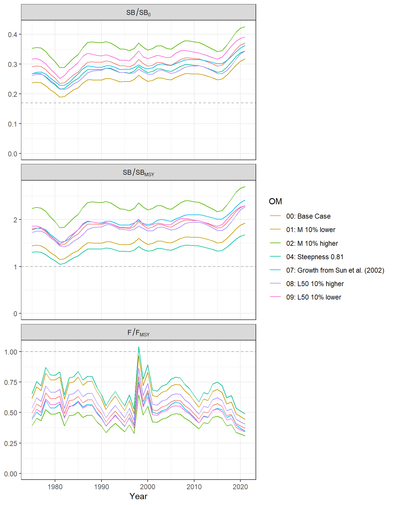
Table 2.4 summarizes the estimated stock status (SB/SB0 & SB/SBMSY), relative fishing mortality (F/FMSY), and the ratio of SBMSY to the equilibrium unfished spawning biomass (SB0), for the Base Case and the 6 sensitivity OMs that are included in the MSE. The MSY-based reference points for each OM are shown in Table 2.5.

Figure 2.4 shows time series plots of SB/SB0, SB/SBMSY, and F/FMSY for the Base Case and the 6 sensitivity OMs.

Table 2.4: Stock status in 2021 (mean over the quarters) for each OM: spawning biomass relative to the equilibrium unfished spawning biomass (SB/SB0) and to SBMSY, fishing mortality relative to FMSY, and SBMSY relative to SB0.

OM	SB/SB0	SB/SBMSY	F/FMSY	SBMSY/SB0
00: Base Case	0.37	2.30	0.37	0.16
01: M 10% lower	0.32	1.93	0.44	0.16
02: M 10% higher	0.43	2.70	0.31	0.16
04: Steepness 0.81	0.34	1.68	0.49	0.21
07: Growth from Sun et al. (2002)	0.36	2.42	0.35	0.15
08: L50 10% higher	0.34	2.27	0.40	0.15
09: L50 10% lower	0.39	2.29	0.34	0.17

Table 2.5: The MSY reference points for each OM. FMSY is the apical fishing mortality (per year) at MSY, SBMSY is female spawning biomass, and MSY is the annual catch.

OM	FMSY	SBMSY (t)	MSY (t)
00: Base Case	0.393	16,629	15,355
01: M 10% lower	0.356	18,317	14,680
02: M 10% higher	0.433	15,487	16,429
04: Steepness 0.81	0.298	23,011	14,735
07: Growth from Sun et al. (2002)	0.416	19,257	15,398
08: L50 10% higher	0.361	14,394	15,125
09: L50 10% lower	0.426	18,640	15,571

Figure 2.4: Historical spawning biomass relative to the equilibrium unfished spawning biomass (top) and to SBMSY (middle), and fishing mortality relative to FMSY (bottom), for each OM. The dashed lines show the LRP (17% SB0), SBMSY, and FMSY.